An investigation of the kinetics of the reaction between titanocene pentasulfide and sulfenyl chloride[1] leading to the formation of the S7 allotrope of sulfur was accompanied by supporting DFT calculations which led to the conclusion that of five possible mechanisms for the reaction, the most probable corresponded to a variant of the concerted σ-bond metathesis (Scheme 1, Mechanism IV, R = Cl). Here we take a closer look at the DFT predictions from the point of view of the impact of continuum solvation on the calculated mechanism.

Scheme 1. Possible reaction mechanisms.
The original study used the new r2scan-3c/Def2-mTZVPP composite DFT functional[2] as implemented in the ORCA 6 program code,[3] for which the (gas phase) mechanistic reported pathway was obtained as shown in scheme 2 below. Here, we re-label the succeeding steps as TS3 and TS4 (see Scheme 3 below, rather than TS2 from scheme 2) to form the final product P, for reasons that will become apparent below.
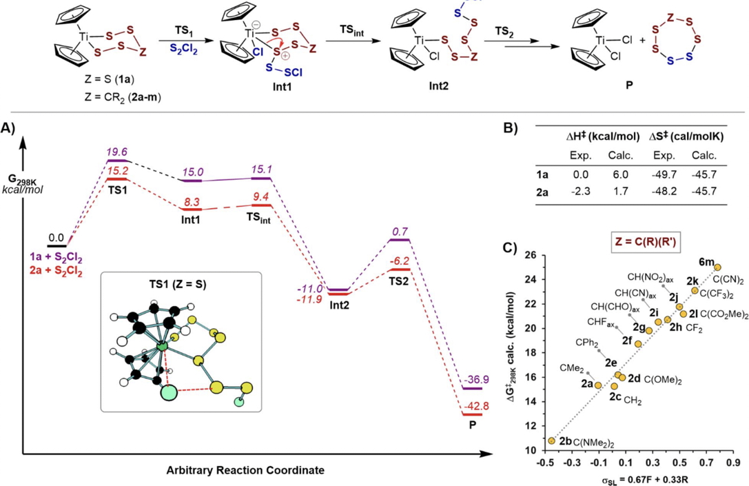
Scheme 2. Reaction scheme and energy profile.[1]
Methodology
In this study, we used an older functional, MN15L[4] for R=Cl (scheme 1), which we have found very effective for the transition elements[5] and which – like r2scan-3c – was designed to be accurate for multi-reference and single-reference systems and for noncovalent interactions, This functional, unlike r2scan-3c, is implemented in the Gaussian 16 program code and hence has the advantage of allowing computed intrinsic reaction coordinate (IRC) data to be usefully visualised using e.g. Gaussview.‡ Transition state geometries were initially obtained from the supporting information given in the original article [1] and re-optimised in the Gaussian program using MN15L/Def2-TZVPP. The thermochemical energies shown in Table A1 were all obtained using GoodVibes[6] (see manual) with an entropic quasi-harmonic treatment frequency cut-off value of 2.0 wavenumbers[7] and an enthalpic quasi-harmonic treatment frequency cut-off value of 50.0 wavenumbers.[8] In the table, harmonic values are indicated as e.g. hG and quasi-harmonic values as qh-G; the difference between these two is relative small. If desired, other harmonic cut-off values can be obtained, as well as at other molar concentrations, using log files obtained from the repository DOIs indicated below, via the command line:
python3 -m goodvibes -q --fs 2 --fh 50 -c 0.0409 logfilename.
Results
Part 1: Gas phase model
The intrinsic reaction coordinate (IRC) deriving from transition state TS1 computed using Gaussian 16, and without inclusion of a solvent continuum model (a gas phase model) is shown below (Table 1, Figure 1).[9] It leads directly to the “half-way” product Int2, with no intervening intermediate such as that shown in Scheme 2 (there labelled Int1[1]). So here, the TS1 IRC conflates the originally reported TS1 and TSint[1] as shown in scheme 2, with the conflation point occuring at an IRC value of ~9. This point can also be seen below as a prominent “hidden intermediate” in the gradient norm plot at the same IRC value. A gradient norm at this point of not quite zero is what makes it a “hidden” rather than a “real” intermediate. The conflation point also ~corresponds to a minimum in the dipole moment plot. Here,[9] the stepsize between points in the IRC calculation was selected as 20 (in units of 0.01 Bohr) and the Hessian was recalculated every 5 steps. The equivalent parameters for the IRCs as noted – but not visualised – in the original article[1] were not stated; it is entirely possible that differences in either these parameters, or the algorithms used to compute the IRC or indeed the use of a different functional could account for this slight difference in behaviour. Slight, because TSint is shown as a very shallow intermediate (Scheme 2[1]).
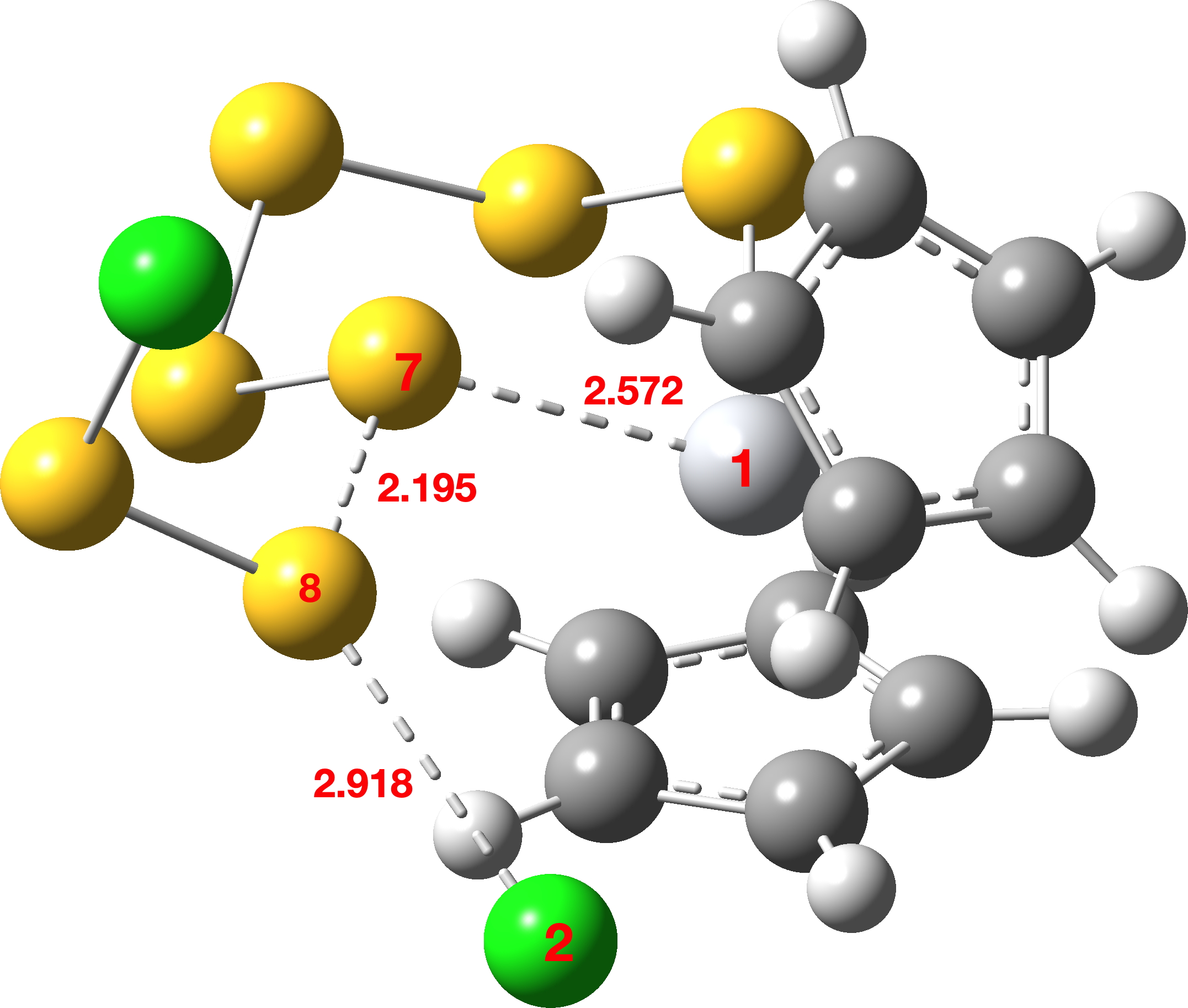
Figure 1. Computed geometry of TS1 in the gas phase at the MN15L/Def2-TZVPP level.
| Table 1. IRC for TS1 in a gas phase MN15L/Def2-TZVPP model. | |
|---|---|
| Total Energy |  |
| Gradient norm |  |
| Dipole moment |  |
Part 2: Continuum solvent model (scheme 3).
FAIR data for all the calculations conducted using a dichloromethane continuum solvent are summarised here, [10] with individual calculations indicated as a reference to a FAIR repository dataset (Table A1). The computed geometry of TS1 changes from the initial values of a) the new S7-S8 bond 2.195 → 2.356Å, b) S8-Cl 2.918 → 2.616Å and c) S7-Ti 2.572 → 2.562Å (Table 2, atom numbering shown in Figure 1).

Scheme 3. Revised reaction scheme showing the formation of the ion-pair Int0 rather than Int1 computed using geometries optimised with continuum solvation effects included.
| Table 2. Calculated geometries for TS1 – Ts4 with solvation | |||
|---|---|---|---|
| # | Geometry | # | Geometry |
| TS1 | 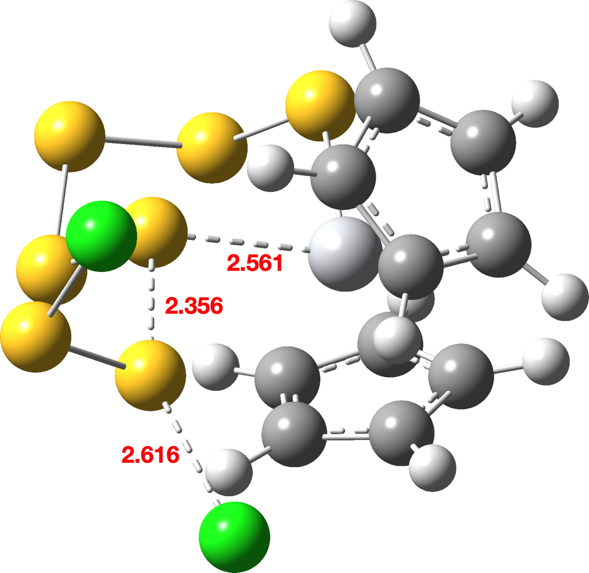 |
Int0 | 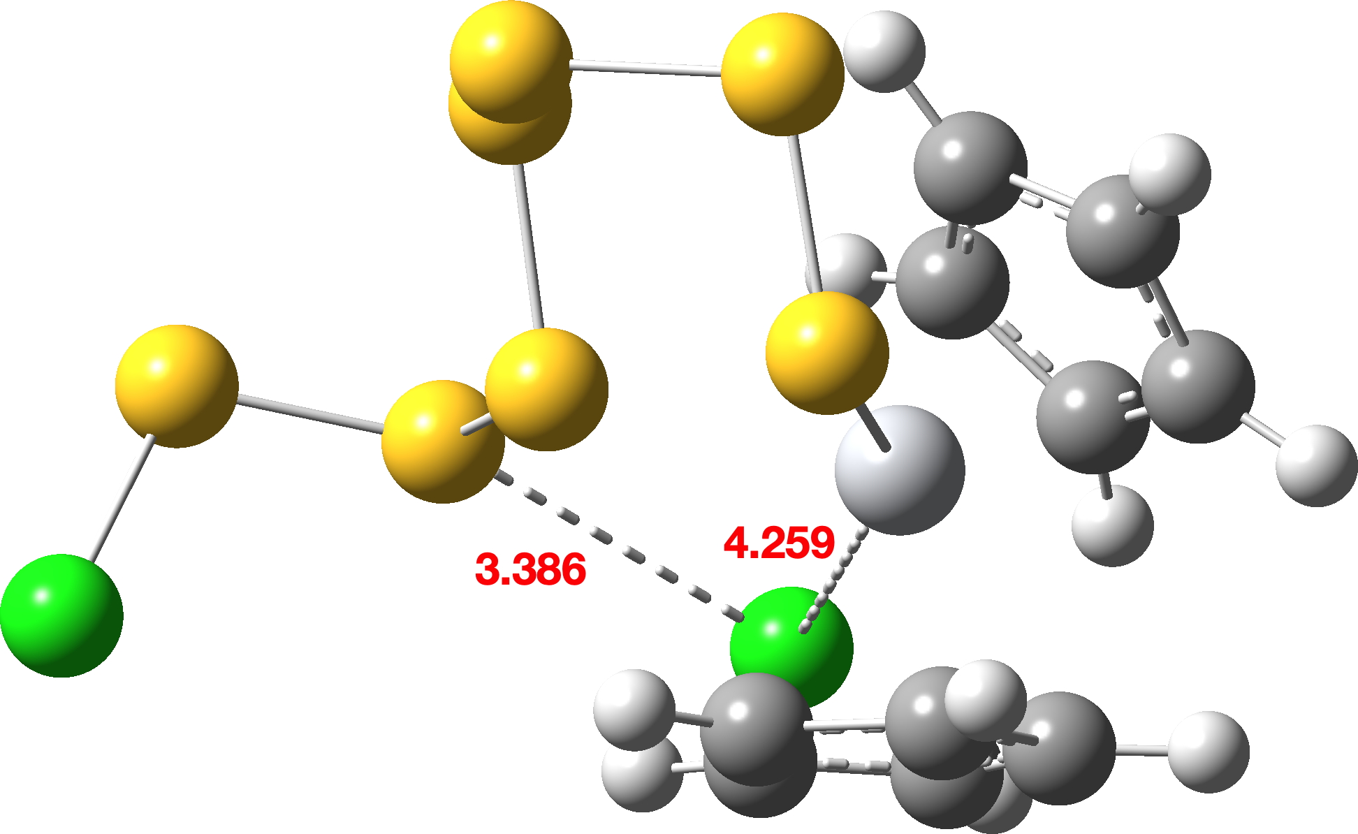 |
| TS2 | 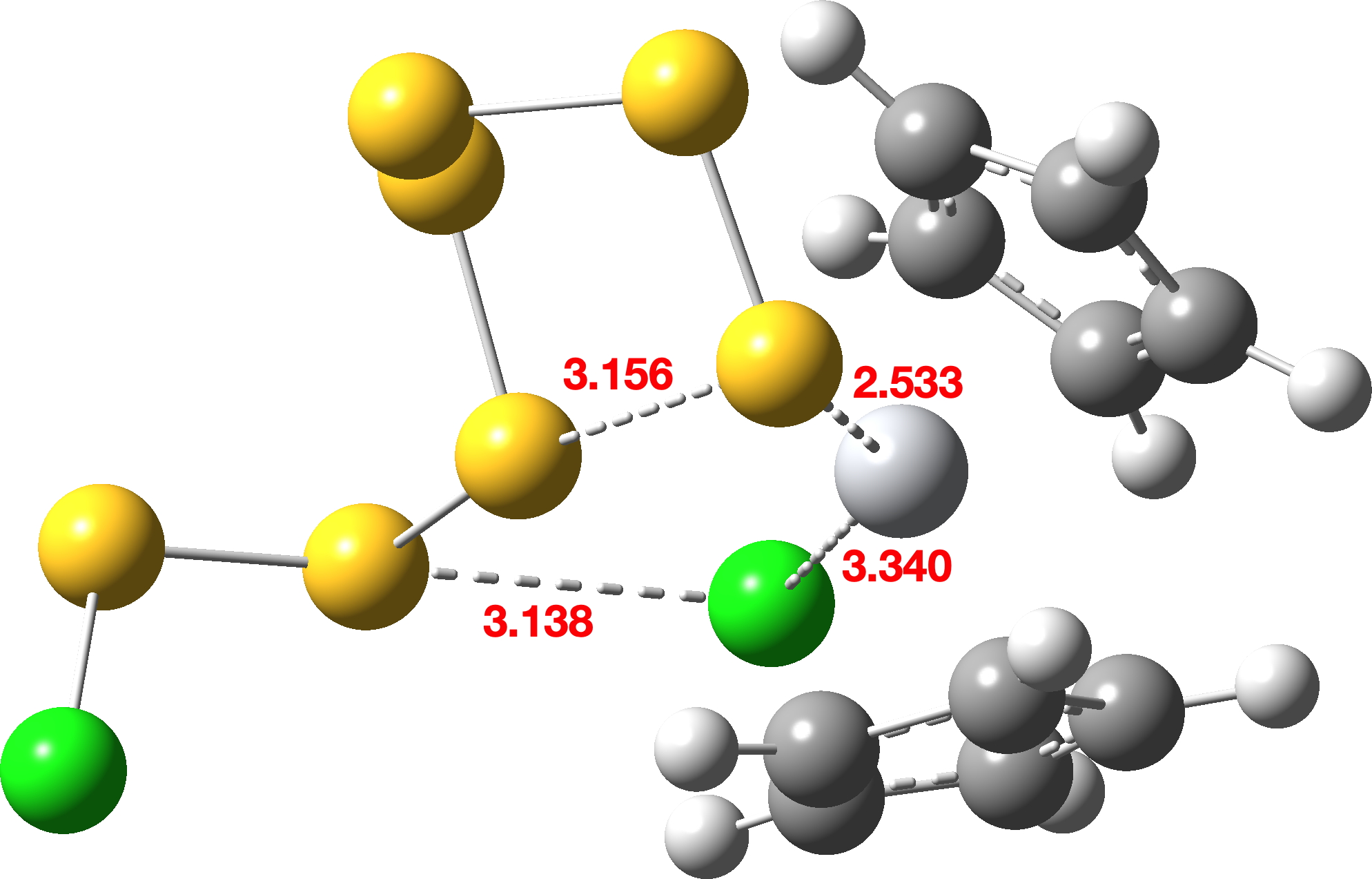 |
Int2 |  |
| TS3 | 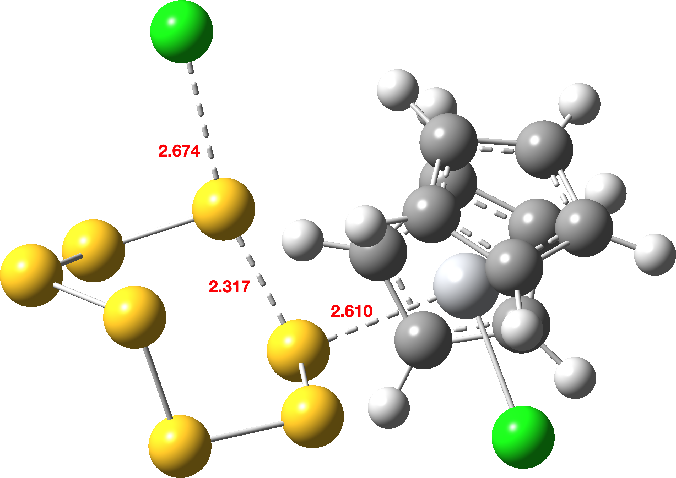 |
TS4 | 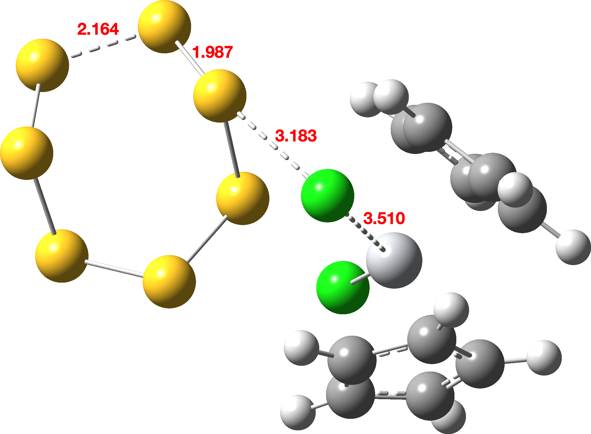 |
When same potential energy surface is computed with a continuum solvent model (Table 3), the “hidden intermediate” present for the gas phase model in the original IRC profile of TS1 (Table 1) now becomes a real ion-pair intermediate (labelled here Int0 in scheme 3 to distinguish it from Int1 in scheme 2) with a discrete chloride anion. Thus Int0 occurs at an IRC value of ~3.5 in the plots below, although it has a very small exit barrier via a transition state, here labelled TS2 (different from the TS2 labelled in scheme 2 above). The plots below (Table 3) are the result of concatenating two separate IRC plots for TS1 and TS2.
| Table 3. IRCs for TS1 + TS2 in a continuum solvent model |
|---|
 |
 |
 |
The gas phase (left) and continuum solvent (right) IRCs are summarised below (Figure 2) to enable a visual comparison of the two potential energy surfaces.
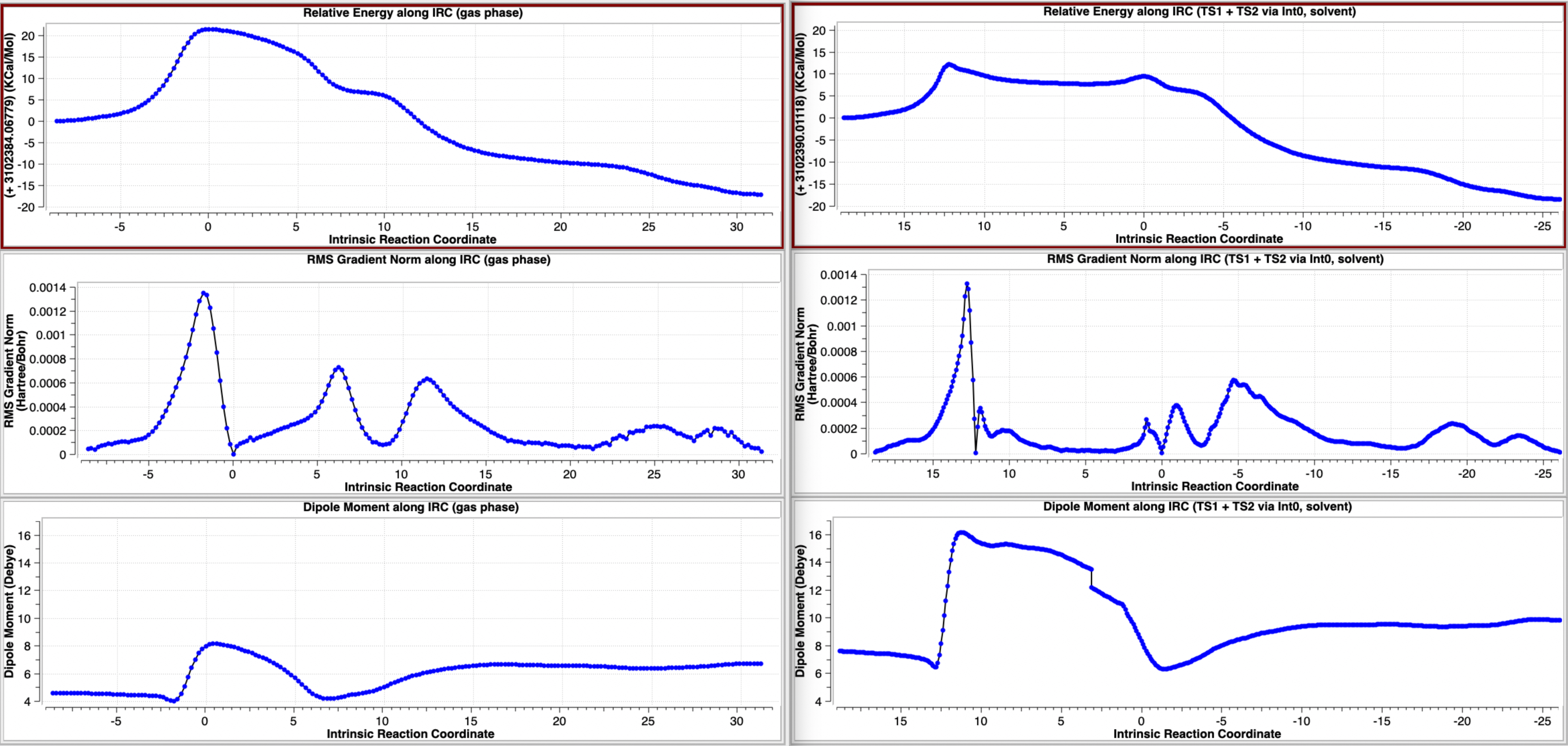
Figure 2. A comparison of the computed IRC energy profiles in the gas phase (left) and continuum dichloromethane solvent (right).
This indicates a change from Mechanism IV under gas phase conditions (scheme 2) to one closer to mechanism II with continuum solvent; an SN2 like displacement of chloride ion at sulfur, followed in a second step by Cl…Ti bond formation and Ti…S cleavage, Scheme 3. This can also be summarised by the following plots of bond lengths in Figure 3.
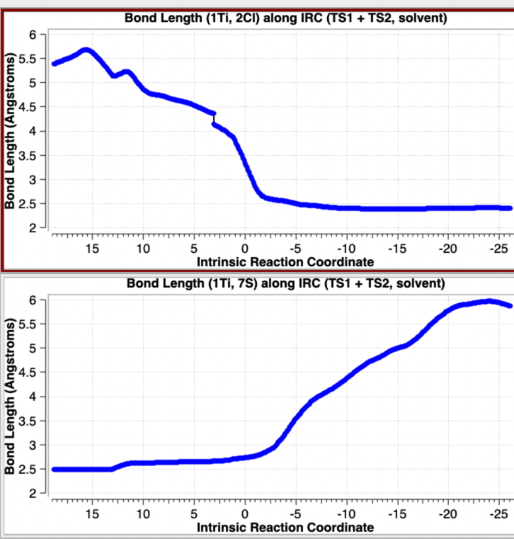
Figure 3. Selected bond length variation for the concatenated IRC profile for TS1 + TS2 in a continuum solvent. See Figure 1 for atom numberings.
The overall results can be summarised in Table 4 indicting that both the original r2scan-3c/Def2-mTZVPP and the MN15L functional used here are both in reasonable agreement with the experimental results obtained from kinetic studies. Also noteworthy is that for substituents such as e.g. 2b, the enthalpy of activation may actually be negative, with the resulting positive value for the free energy of activation being a consequence of a very negative entropy of activation.
| Table 4. Solvent DCM model: Mechanism II through to Ion-Pair intermediate Int0 rather than the original Int1. | |||
|---|---|---|---|
| Source | ΔH | ΔS | ΔG |
| 1a: Article | 6.0 | -45.7 | 19.6 |
| 1a: This work | 3.4 | -31.5 | 12.8 |
| 1a: Expt/1M | 0.0 | -49.7 | 14.8 |
| 2a: Article | 1.7 | -45.7 | 15.3 |
| 2a: This work | 0.8 | -39.5 | 12.6 |
| 2a: Expt/1M | -2.3 | -48.2 | 12.6 |
| 2b: Article | ~10.8 | ||
| 2b: This work | -1.4 | -34.1 | 8.80 |
| 6m: Article | ~25.0 | ||
| 6m: This work | 8.95 | -39.2 | 20.6 |
Conclusions
The overall conclusion is simple; when the possibility of ion-pair formation on a reaction potential energy surface is present, it matters how the geometries of all the species involved are obtained. A gas phase geometry optimised model is likely to disfavour the formation of such an ion-pair, whereas a continuum solvent geometry optimised model is more likely to promote such species. This effect can be seen especially in Figure 2, where the two potentials are shown side by side. Such promotion of ion-pairs is likely to reduce any concerted behaviour of the reaction into a two-stage stepwise process. Thus the concerted nature of mechanism IV (Scheme 1) morphs into more stepwise behaviour (Mechanism II, Scheme 1 modified as in Scheme 3). Overall however, while the resulting calculated energetic barriers, although reduced by inclusion of solvation, are unlikely provide definitive evidence of which mechanism actually prevails, the greater change in dipole moment in the stepwise behaviour is more consistent with the experimentally observed effects of solvent identity on the rate.
Appendix
All energies for the computed species, obtained with optimisation with a dichloromethane continuum solvent model. Values for the default concentration of 0.0409M are shown for completeness and to enable facile reconciliation with those included in the published FAIR datasets.
| Table A1. Calculations at the MN15L/Def2-TZVPP; Def2-QZVPP on Ti/CPCM=Dichloromethane level with geometry optimisation. | ||||||
|---|---|---|---|---|---|---|
| 1a (scheme 2) | ||||||
| Species | h-H | T.h-S | h-G | qh-H | T.qh-S | qh-G |
| Z=S | -3227.1212a -3227.1212b |
0.05845 0.05543 |
-3227.179639 [11] -3227.176621 |
-3227.12140 -3227.12140 |
0.05845 0.05543 |
-3227.17985 -3227.17683 |
| S2Cl2 | -1716.63131a -1716.63135b |
0.03637 0.03335 |
-1716.667668 [12] -1716.664658 |
-1716.63135 -1716.63135 |
0.03637 0.03335 |
-1716.66771 -1716.66470 |
| Sum | -4943.75254a -4943.75254b |
0.09481 0.08878 |
-4943.847307 -4943.841279 |
-4943.75275 -4943.75275 |
0.09481 0.08878 |
-4943.84756 -4943.84152 |
| TS1 | -4943.74534a -4943.74534b |
0.07984 0.07682 |
-4943.825172 [13] -4943.822153 |
-4943.74734 -4943.74734 |
0.07984 0.07682 |
-4943.82717 -4943.82415 |
| ΔTS1 | 4.52 | -31.53 | 13.88 | 3.39 | -31.52 | 12.79 |
| ΔTS1b | 4.52 | -25.17 | 12.00 | 3.39 | -25.17 | 10.90 |
| Int0c | -4943.75128 | 0.08039 | -4943.831670 [14] |
-4943.75298 | 0.08039 | -4943.83337 |
| ΔInt0 | 0.76 | -30.36 | 9.81 | -0.15 | -30.36 | 8.91 |
| TS2 | -4943.74951 | 0.07801 | -4943.827519 [15] |
-4943.75100 | 0.07801 | -4943.82901 |
| ΔTS2 | 1.88 | -35.33 | 12.42 | 1.10 | -35.36 | 11.64 |
| Int2 | -4943.79255 | 0.08031 | -4943.872859 [16] |
-4943.79432 | 0.08031 | -4943.87463 |
| ΔInt2 | -25.13 | -30.53 | -16.03 | -26.09 | -30.53 | -16.99 (-11.0 lit) |
| TS3 | -4943.77886 | 0.08003 | -4943.858887 [17] |
-4943.78065 | 0.08003 | -4943.86068 |
| ΔTS3 | -16.54 | -30.12 | -7.27 | -4943.78065 | -8.23 | |
| Int3 | -4943.78456 | 0.079887 | -4943.864446 [18] |
-4943.78619 | 0.079887 | -4943.86607 |
| ΔInt3 | -20.12 | -31.42 | -10.76 | -20.98 | -31.42 | -11.62 |
| TS4 | -4943.78439 | 0.07807 | -4943.862461 [19] |
-4943.78599 | 0.07807 | -4943.86406 |
| ΔTS4 | -20.01 | -35.23 | -9.51 | -20.86 | -35.23 | -10.36 |
| S7 as product | -2787.10568 | 0.04667 | -2787.152347 [20] |
-2787.10608 | 0.04667 | -2787.15275 |
| Cp2TiCl2 | -2156.70450 | 0.04990 | -2156.754401 [21] |
-2156.70456 | 0.04990 | -2156.75447 |
| Product P | -4943.81017 | 0.09657 | -4,943.906749 | -4943.81064 | 0.09657 | -4,943.90722 |
| ΔProduct P | -36.19 | 3.70 | -37.30 | -36.33 | 3.70 | -37.43 (-36.9 lit) |
| 2a: | ||||||
| Z=CMe2 | -2946.72598a -2946.72598b |
0.06683 0.063808 |
-2946.7928059 [22]–2946.789786 |
-2946.72674 -2946.72674 |
0.06683 0.063806 |
-2946.79356 -2946.790542 |
| S2Cl2 | -1716.63131a -1716.63135b |
0.03637 0.03335 |
-1716.667668 [12] -1716.664658 |
-1716.63135 -1716.63135 |
0.03637 0.03335 |
-1716.66771 -1716.66470 |
| Sum | -4663.35729 -4663.35729 |
0.10319 0.097158 |
-4663.4604739 -4,663.454444 |
-4663.35808 -4663.35808 |
0.10319 0.097156 |
-4663.46127 -4663.455242 |
| TS1 | -4663.35477a -4663.35477b |
0.08445 0.081429 |
-4663.439222 [23]-4663.436203 |
-4663.35677 -4663.35677 |
0.08445 0.081429 |
-4663.44122 -4663.438201 |
| ΔTS1a | 1.58 | -39.45 | 13.34 | 0.82 | -39.46 | 12.59 |
| ΔTS1b | 1.58 | -33.10 | 11.45 | -33.10 | 10.69 | |
| TS2 | -4663.36425 | 0.08207 | -4663.446325 [24] |
-4663.36574 | 0.08207 | -4663.44782 |
| ΔTS2 | -4.37 | -44.44 | 8.88 | -4.80 | -44.44 | 8.44 |
| 2b: | ||||||
| Z=C(NMe2)2 | -3135.79512 -3135.79512 |
0.07575
0.072730 |
-3135.870870 [25]-3135.867852 |
-3135.79611 -3135.79611 |
0.07575 0.072730 |
-3135.87186 -3135.86884 |
| S2Cl2 | -1716.63131a -1716.63135b |
0.03637 0.03335 |
-1716.667668 [12] -1716.664658 |
-1716.63135 -1716.63135 |
0.03637 0.03335 |
-1716.66771 -1716.66470 |
| Sum | -4852.4264 -4852.4264 |
0.11212 0.10608 |
-4852.538538 -4852.53251 |
-4852.42745 -4852.42745 |
0.11212 0.10608 |
-4852.5396 -4852.53354 |
| TS1 | -4852.42719 -4852.42719 |
0.09602 0.09300 |
-4852.523215 [26] -4852.520196 |
-4852.42964 -4852.42964 |
0.09591 0.09289 |
-4852.52555 -4852.522536 |
| ΔTS1a | -0.49 | -33.86 | 9.62 | -1.37 | -34.11 | 8.80 |
| ΔTS1b | -0.49 | -27.53 | 7.27 | -1.37 | -27.76 | 6.91 |
| TS2 | -4852.43669 | 0.09143 | -4852.528126 [27] |
-4852.43823 | 0.09143 | -4852.52966 |
| ΔTS2 | -6.44 | -43.54 | 6.53 | -6.76 | -43.54 | 6.22 |
| 6m: | ||||||
| Z=C(CN)2 | -3052.59951 -3052.59951 |
0.06956 0.06654 |
-3052.669074 [28] -3052.666055 |
-3052.60050 -3052.60050 |
0.06956 0.06654 |
-3052.67007 -3052.66705 |
| S2Cl2 | -1716.63131a -1716.63135b |
0.03637 0.03335 |
-1716.667668 [12] -1716.664658 |
-1716.63135 -1716.63135 |
0.03637 0.03335 |
-1716.66771 -1716.66470 |
| Sum | -4769.23082 -4769.23082 |
0.10593 0.09989 |
-4769.336742 -4769.330713 |
-4769.23185 -4769.23185 |
0.10593 0.09989 |
-4769.3378 -4769.33175 |
| TS1 | -4769.21540a -4769.21540b |
0.08731 0.08423 |
-4769.30271 [29] -4769.29970 |
-4769.21759 -4769.21759 |
0.08731 0.08423 |
-4769.30490 -4769.30188 |
| ΔTS1a | 9.68 | -39.18 | 21.36 | 8.95 | -39.18 | 20.63 |
| ΔTSb | 9.68 | -32.83 | 19.46 | 8.95 | -32.83 | 18.74 |
| TS2 | -4769.22451 | 0.08582 | -4769.310328 [30] |
-4769.22626 | 0.08582 | -4769.31208 |
| ΔTS2 | 3.96 | -42.32 | 16.58 | 3.51 | -42.32 | 16.13 |
a0.0409M b1.0M cInt0 is ion pair comprising S+ and Cl– See Table 3 and scheme 3.
Footnotes
‡Currently at least, Gaussian is better supported by associated visualisation programs then ORCA.
This post has DOI: 10.59350/1a48f-rj714
Authors
References
- P.H. Helou de Oliveira, P.J. Boaler, G. Hua, N.M. West, R.T. Hembre, J.M. Penney, M.H. Al-Afyouni, J.D. Woollins, A. García-Domínguez, and G.C. Lloyd-Jones, "Kinetics of sulfur-transfer from titanocene (poly)sulfides to sulfenyl chlorides: rapid metal-assisted concerted substitution", Chemical Science, vol. 15, pp. 11875-11883, 2024. https://doi.org/10.1039/d4sc02737j
- S. Grimme, A. Hansen, S. Ehlert, and J. Mewes, "r2SCAN-3c: A “Swiss army knife” composite electronic-structure method", The Journal of Chemical Physics, vol. 154, 2021. https://doi.org/10.1063/5.0040021
- F. Neese, F. Wennmohs, U. Becker, and C. Riplinger, "The ORCA quantum chemistry program package", The Journal of Chemical Physics, vol. 152, 2020. https://doi.org/10.1063/5.0004608
- H.S. Yu, X. He, and D.G. Truhlar, "MN15-L: A New Local Exchange-Correlation Functional for Kohn–Sham Density Functional Theory with Broad Accuracy for Atoms, Molecules, and Solids", Journal of Chemical Theory and Computation, vol. 12, pp. 1280-1293, 2016. https://doi.org/10.1021/acs.jctc.5b01082
- E.M. Richards, L. Casarrubios, J.M. D'Oyley, H.S. Rzepa, A.J.P. White, K. Goldberg, F.W. Goldberg, J.A. Bull, and S. Díez‐González, "Bidentate NHC‐Containing Ligands for Copper Catalysed Synthesis of Functionalised Diaryl Ethers", Advanced Synthesis & Catalysis, vol. 367, 2024. https://doi.org/10.1002/adsc.202400909
- I. Funes-Ardoiz, and R.S. Paton, "GoodVibes: version 2.0.3", 2018. https://doi.org/10.5281/zenodo.1435820
- S. Grimme, "Supramolecular Binding Thermodynamics by Dispersion‐Corrected Density Functional Theory", Chemistry – A European Journal, vol. 18, pp. 9955-9964, 2012. https://doi.org/10.1002/chem.201200497
- Y. Li, J. Gomes, S. Mallikarjun Sharada, A.T. Bell, and M. Head-Gordon, "Improved Force-Field Parameters for QM/MM Simulations of the Energies of Adsorption for Molecules in Zeolites and a Free Rotor Correction to the Rigid Rotor Harmonic Oscillator Model for Adsorption Enthalpies", The Journal of Physical Chemistry C, vol. 119, pp. 1840-1850, 2015. https://doi.org/10.1021/jp509921r
- H. Rzepa, "TS1 Cp2TiS5 + S2Cl2, gas phase, Def2-QZVPP on Ti, G = -4943.798931 IRC", 2025. https://doi.org/10.14469/hpc/15219
- H. Rzepa, "Mechanism of reaction between titanocene pentasulfide and sulfenyl chloride", 2025. https://doi.org/10.14469/hpc/15204
- H. Rzepa, "CYPTIS5 Def2-QZVPP on Ti, TZVPP on rest G = -3227.179639 (Def2-TZVPP = -3227.141839)", 2025. https://doi.org/10.14469/hpc/15150
- H. Rzepa, "S2Cl2, G = -1716.667668", 2025. https://doi.org/10.14469/hpc/15196
- H. Rzepa, "TS1 for Sn2 by S on S-Cl Def2-QZVPP on Ti, G = -4943.825172 (TS2 -4943.827519)", 2025. https://doi.org/10.14469/hpc/15179
- H. Rzepa, "Ion pair Int0 SCRF(CPCM), G = -4943.831670", 2025. https://doi.org/10.14469/hpc/15205
- H. Rzepa, "TS2 Def2-QZVPP on Ti, TZVPP on rest G = -4943.827519", 2025. https://doi.org/10.14469/hpc/15154
- H. Rzepa, "TS2, IRC => Int2, G = -4943.872859", 2025. https://doi.org/10.14469/hpc/15206
- H. Rzepa, "C2pTiS5. TS3, second SN2 with Def2-QZVPP on Ti, G = -4943.858887", 2025. https://doi.org/10.14469/hpc/15248
- H. Rzepa, "C2pTiS5. TS3, second SN2 with Def2-QZVPP on Ti ==> Int3 G = -4943.859300 ==> Int3 G =0.106 oz -4943.864446", 2025. https://doi.org/10.14469/hpc/15254
- H. Rzepa, "Cp2TsS5 + S2Cl2, TS4, G = -4943.862461", 2025. https://doi.org/10.14469/hpc/15251
- H. Rzepa, "C2pTiS5. Final Product, G = -4943.902398 S7 -2787.152347", 2025. https://doi.org/10.14469/hpc/15578
- H. Rzepa, "C2pTiS5. Final Product, G = -4943.902398 Cp2TiCl2 G =-2156.754402 + -2787.152347 = -4,943.906749", 2025. https://doi.org/10.14469/hpc/15579
- H. Rzepa, "2a, Def2-QZVPP on Ti, G = -2946.7928059", 2025. https://doi.org/10.14469/hpc/15193
- H. Rzepa, "TS2 for Sn2 by S on S-Cl Def2-QZVPP on Ti, G = -4943.825172 (TS1 -4943.827519) => 2a G = -4663.439222", 2025. https://doi.org/10.14469/hpc/15195
- H. Rzepa, "TS1, Def2-QZVPP on Ti, TZVPP on rest G = -4943.827519 => 2a G = -4663.446325", 2025. https://doi.org/10.14469/hpc/15194
- H. Rzepa, "2b CYPTIS4C(NMe2)2 G = -3135.870870", 2025. https://doi.org/10.14469/hpc/15197
- H. Rzepa, "TS2 for Sn2 by S on S-Cl Def2-QZVPP on Ti, => 2b G = -4852.523215", 2025. https://doi.org/10.14469/hpc/15199
- H. Rzepa, "TS1, Def2-QZVPP on Ti, TZVPP on rest G = -4943.827519 => 2b G = -4852.528126", 2025. https://doi.org/10.14469/hpc/15198
- H. Rzepa, "6m. CYPTIS4C(CN)2 G = -3052.669074", 2025. https://doi.org/10.14469/hpc/15200
- H. Rzepa, "TS2 for Sn2 by S on S-Cl Def2-QZVPP on Ti, => 6m G = -4769.302718", 2025. https://doi.org/10.14469/hpc/15203
- H. Rzepa, "TS1, Def2-QZVPP on Ti, TZVPP on rest => 6m", 2025. https://doi.org/10.14469/hpc/15201