Techniques of Molecular Modelling: Transition States

1. Single bond rotations, preserving the 2-electron character of the bond (i.e. dihedral driving), and angle deformations which do not change electronic character at the atoms
2. Bond formation/cleavages which predominantly follow the two-electron "arrow pushing" formalisms (wavefunction dominated by a single configuration comprising doubly filled molecular orbitals) and which can be handled by Hartree-Fock models. If such arrow pushing results in charge separation (or its loss), then solvation models will have to be added.
3. Bond formation/cleavages and double bond rotations, where two-electron arrow pushing is not followed (homolytic bond cleavage, asynchronous bond cleavage/rotation forming biradicals) in which the wavefunction comprises two or more electronic configurations whose relative contributions change as the reaction proceeds. These are known as multi-configuration (MCSCF) reference states.
4. More complex points in the potential surface which include regions where different electronic (excited) states meet (conical intersections), and where the molecular dynamics (trajectories) of the atoms controls the reactions as well as simply the potential energy surfaces

Molecular mechanics can sometimes be used for 1 above, but molecular orbital methods have to be used for the rest of these cases.

Case Study 6: The transition state approach for aromatic electrophilic substitutions

The previous approach, which relied on the Hammond postulate to infer the properties of the transition state for the reaction is indirect. A better approach is to locate the actual transition state. The easiest way of doing this is to define one bond, in this case the distance between the N of a NO₂⁺ ion and the carbon it attaches to in an aromatic ring) as a reaction coordinate, and calculate the (Quantum mechanical) energy of the system as a function of this bond length. In the schematic energy profile so obtained, point 1 shows the nitronium ion forming a weak π-π complex with the aromatic in which the ion and the aromatic are face-to-face in their relative orientation. Transition state 2 is the highest in energy; point 3 represents the geometry of the "Wheland" intermediate. At this point, one has to select a different reaction coordinate, and one can now complete the the reaction via transition state 4, going to final product 5.

Case study 6 continued: The Transition states

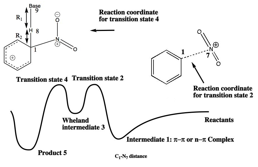
From this reaction profile, one can select the approximate geometry of the transition 2 or 4 and use a precise algorithm such as Eigenvector Following to fully optimise its geometry. This is then subjected to a calculation of the 2nd derivatives of the energy with respect to the (3N) coordinates of the molecule. This matrix is diagonalised, and shown to have all positive roots (eigenvalues) except ONE. This is the reaction coordinate normal mode. The eigenvalue energy can be converted to a vibrational frequency, and the eigenvectors of this root of the matrix can be visualised (animated).

This procedure was followed for Pyridine rather than benzene (see see DOI: 10.1021/ja021152s for details of calculations for the prototypic reaction of a nitronium ion with benzene, where less is more, i.e. this simple prototype is in fact quite complex). The reaction coordinate normal mode obtained for the transition state clearly shows the required C-N bond formation in the 3-position.

The Wheland intermediate must now break down by proton removal to form the final product. This too should be studied by the transition state model, using the C-H and H-base distances as a reaction coordinate. Only then can one determine whether the C...N bond formation, the C...H bond cleavage, or a synchronous combination of both is actually the rate determining or highest energy step in the pathway.

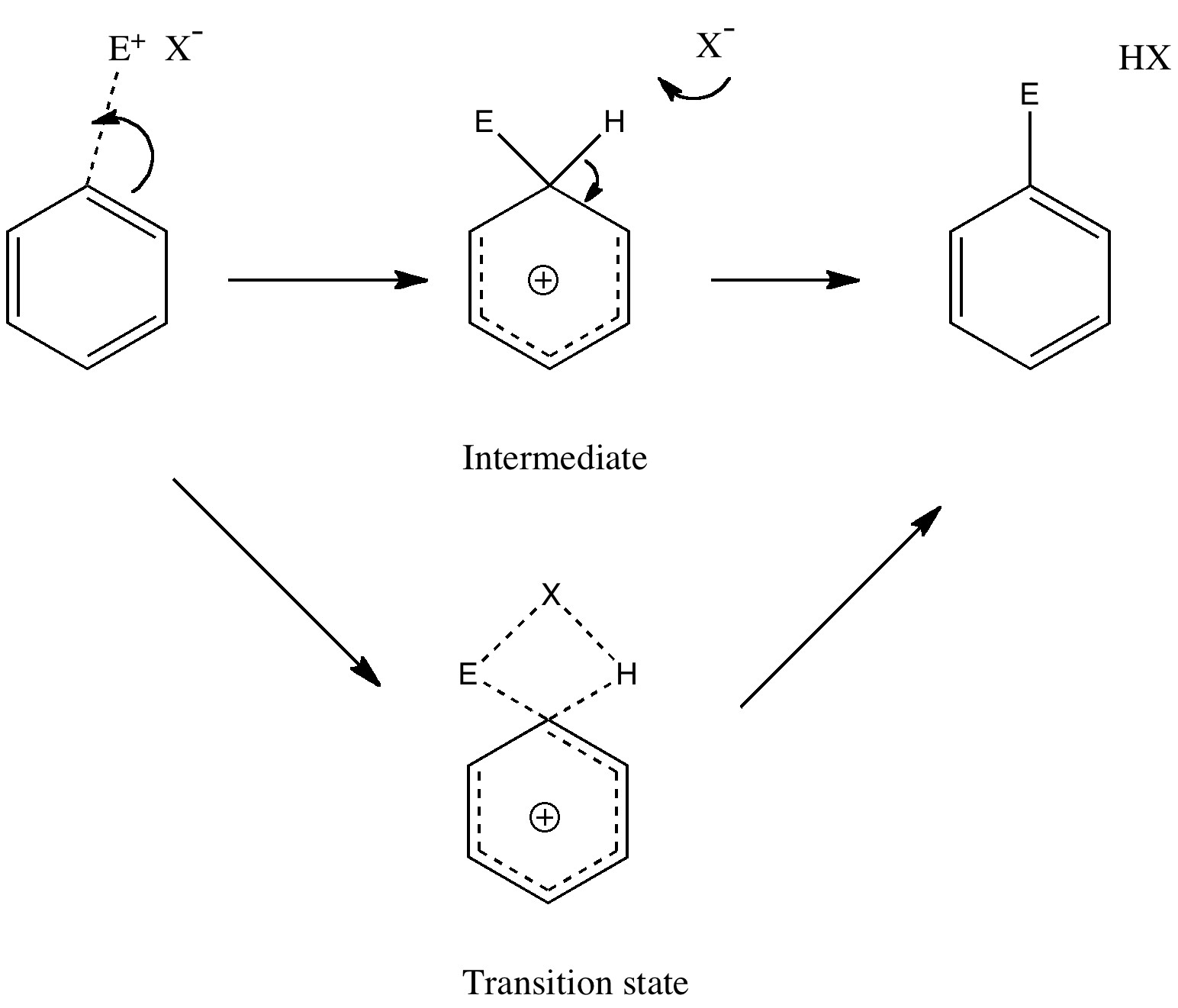
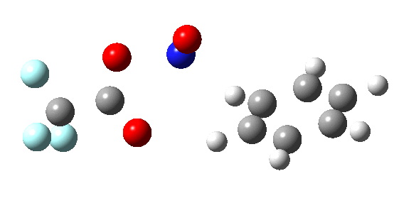
If the electrophile is voracious, it tends to seek to acquire electrons as quickly as possible. This can favour Wheland intermediates (provided they are not destabilized, as above), as with E-X= CF₃CO₂F (E⁺=F⁺) for which an intrinsic reaction coordinate is shown below:

If the electrophile E⁺ is less voracious, and has a counterion X^- which can act as the required base, it is perfectly possible for the Wheland intermediate to vanish entirely. Such merging of the two transition states and one intermediate into a single concerted pathway showing just a single transition state is shown below in the form of an intrinsic reaction coordinate (IRC), which charts the energy of the system as a function of the degree of reaction for E⁺=NO⁺ and X=CF₃CO₂^-;

Aromatic electrophilic substitution as part of a catalytic process

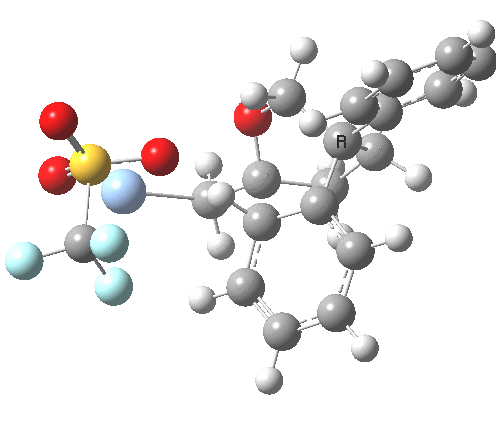
An real example of such a reaction profile is found in the mechanism of metal-catalysed ring closure as shown below. Here would involve the attack by an electrophilic carbon on the carbon of phenyl group as illustrated with the red arrow below. In this mechanism, the electrophilic C-C bond formation (TS2) is actually concurrent with the proton removal by the metal ligand (TS4), i.e. TS2 and TS4 are one and the same, and the Wheland intermediate has no existence! By combining the two steps, the molecule does its best to avoid loss of too much aromaticity, which the existence of a discrete Wheland intermdiate would imply.

See DOI: http://dx.doi.org/10.1039/b913295c and this blog post for more details

Case Study 5: Revisited. The Diels-Alder transition state

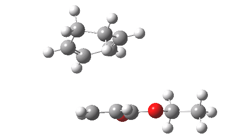
This involved the catalysis of the Diels-Alder reaction inside the cavity of a crystal. An interesting question to ask is how the transition state is influenced by the surrounding cavity. We can use the above approach to locate this transition state both outside and inside the cavity.

Unlike the transition state for electrophilic aromatic nitration, the Diels-Alder has TWO bonds forming. The above approach could be extended by performing a two-dimensional reaction path search, varying the length of both bonds systematically to construct a 2D map. However, experience shows one can in fact adopt a short cut. It turns out that very many C-C bond forming reactions show a C-C bond length in the region 2.1-2.3Å. A good approximation is to calculate just the single point in the 2D map by restraining both forming C-C bonds to 2.2Å, whilst fully minimising all the remaining geometric variables (in practice this is done in the Gaussian program by specifying the keyword opt=modredundant and adding the two bond specifications at the end of the geometry input).

In the second step, the precise values of the two C-C bonds can now be themselves optimised by the Eigenvector Following method, involving calculating the force constant (Hessian) matrix (keyword opt(calcfc,ts)). This matrix is now quite likely to have a single negative root, as a consequence of having pre-optimised the geometry with the two C-C bonds constrained, and the EF method in effect implements the constraints that the energy of the total system will be maximised by following the vectors of this single (-ve) root, whilst simultaneously minimising the energy for all the other (+ve) 3N-7 roots of the Hessian. This argument of course presupposes that BOTH bonds have a length of 2.1-2.3Å at the transition state. Whilst simple Diels-Alders are so symmetrical, the topic has been controversial in the past, and there is good reason to suppose that larger cycloadditions such as e.g. _π6_s + _π8_s may be very unsymmetrical (DOI: 10.1021/ja00768a085). The result can be seen below for the and Diels-Alder transition states.

One interesting question to ask; how does the cavity affect the properties of the transition state. Thus outside the cavity, the transition state procedure (ωB97XD/6-31G(d) predicts that the two C-C bonds forming are 2.11 and 2.47Å, some small asymmetry tending towards a zwitterionic transition state with a C^- stabilized by an adjacent ester group and a carbocation stabilised by allylic resonance. In the cavity the bond lengths are 2.13 and 2.50Å, indicating that the cavity does indeed have a small influence on the reaction enclosed within it (in effect acting as solvent). The point is further emphasized by the values of ΔH^‡ and ΔG₂₉₈^‡:

System	ΔH‡	ΔG‡
Isolated reaction	15.5	29.5
Cavity reaction	16.5	20.0

Using Ln k/T = 23.76 – ΔG/RT and t_1/2 = Ln 2/k; 20.0 kcal/mol corresponds to a half life of ~40 hour at room temperature (298K), more or less what is observed. For more details, see here.