Techniques of Molecular Modelling: Molecular Orbital Methods

Molecular orbital methods date back to the origins of quantum mechanics and the Schroedinger equation. The first practical chemical solution to this equation was formulated by Erich Huckel in 1931 and dealt exclusively with planar conjugated systems. The theory was extended by Hartree and Fock, Pauling, Mulliken and others, and implemented in the 1960s by Hoffmann to all valence electron systems, by Pople and others in the 1970s to semi-empirical methods (AM1 due to Dewar, PM3 and 6 due to Stewart, PDDG due to Jorgensen etc) and to ab initio/density functional methods (Gaussian, etc) in the 1980s. In essence, MO methods differ from the molecular mechanics methods in providing explicit solutions for the electronic component of a molecule rather than just the nuclear terms.

A Quick Summary of the Principle Molecular Orbital Methods used today

Methods which integrate Hamiltonian and Basis set AM1 (Austin Model 1, based on a parametrised Hartree-Fock model), a Semiempirical method parametrised for 42 elements. The method uses only valence shell atomic orbitals, representing them with Slater functions (see below), whilst the inner shells (e.g. 1s for C) and other terms in the Hartree-Fock equations are modelled with parametric functions (often referred to as the NDDO set of approximations) in a manner similar to molecular mechanics. PM3, a reparametrisation of AM1, introduced in 1989 and a bit like the curate's egg (much better for e.g. H-bonding). Parameters for 42 elements in all combinations. PM6, a reparametrisation of PM3 introduced in 2007 and about twice as accurate. Includes parameters for 69 elements (but not necessarily all possible combinations) DOI: 10.1007/s00894-007-0233-4. RM1 is the latest method in this stable,offering high accuracy parameters for all combinations of the 10 most common elements (H, C, N, O, P, S, F, Cl, Br, I). Oniom: A method first introduced in 1996 which partitions a molecule into layers, each treated using a different approximation. The most common is a two layer model, the outer layer treated using molecular mechanics (or even a simpler unified field model), the inner one treated using MO theories. Three layer models apply one of mechanics, one of semi-empirical and one of ab initio MO theories (DOI: 10.1021/jp962071j)
List of Ab initio/Density functional Hamiltonians	List of Basis sets
RHF, or (Spin) Restricted Hartree Fock. Applied to singlet electronic states (all electrons paired) and used for relatively rapid prototyping of a calculation. No consideration for electron correlation. UHF, or (Spin) Unrestricted Hartree Fock, for use with open shell systems (doublets, triplets, etc). ROHF. Restricted openshell Hartree Fock, for open shell systems. More limited than UHF for some systems (ie 2nd derivatives, etc) but free of spin contamination. B3LYP (UB3LYP): A popular density functional method (not strictly an ab initio one), offering good reliability and electron correlation treatment at the penalty of about half the speed of a RHF calculation. There are many other functionals that have been proposed, but none tested so thoroughly as this one. These are good for so-called "short range" correlation effects. DFT-D (Density functional theory with empirical van der Waals Corrections; DOI: 10.1039/b615319b). These dispersion corrections have been incorporated into new generations of double-hybrid methods, such as BML and B2-PLYP/B2GP-PLYP which address many deficiencies of B3LYP (DOI: 10.1021/jp710179r) and which occupy the so-called fifth rung of Jacob's ladder of approximations (DOI: 10.1063/1.1390175) MP2 (MP4), Moller-Plesset methods based on perturbation theory, an older method than the density functionals for incorporating electron correlation. Perhaps 10-100 times slower than HF, but in some cases more reliable, especially for so-called "long range correlation effects". New double-hybrid DFT methods rely on MP2 for the correlation part of the DFT functional. CISD; Configuration Interaction based on a Hartree-fock reference state, for systems where multiple electronic configurations and electron correlation are important, e.g. excited states etc. CASSCF(n,n); a keyword for invoking multi-configurational SCF where the Hartree-Fock reference state is simply not good enough (i.e. transition metal series, excited states, etc). CCSD(T), CCSDTQ; the so-called coupled-cluster approach to the correlation problem. Very very expensive, and can only be properly applied to about 10-12 (non-hydrogen) atoms.	STO-3G. A minimal (single-ζ) basis set. Use for very rapid prototyping of a calculation, or initial geometry optimisation from a poor starting guess. The 3 means using three Gaussian-type functions sharing a common exponent (ζ) to represent a shell (modelled on the Slater-type-function or STO, this being adapted from the Schroedinger solutions for a hydrogen atom). 3-21G. a small double-ζ basis set due to Pople, and available for most of the periodic table (see Tech info and particularly the section on basis sets). The 3 is used for the core electrons (1s for eg carbon), the "2" and "1" are used for the valence electrons, and are represented by respectively two and one Gaussian functions, each with its own ζ exponent. The "" means polarization (d) functions on e.g. S, P, Cl etc. Used for relatively rapid prototyping of a calculation. SDD, an alternative basis set for the entire period table using effective core potentials (Pseudopotentials) to reduce the number of basis functions (for the core electrons) and to include relativistic effects (for heavy elements). 6-31+(d,p). A reasonably high quality double-ζ basis set with anionic diffuse (+) and "polarisation functions" on the atoms ("p" orbital for Hydrogen, "d and f" orbital for carbon, "f and g" orbital for transition metals, etc). cc-pVTZ. A triple-ζ correlation-consistent basis set with valence polarization functions, now regarded as appropriate for reasonably high quality on small to medium sized molecules. aug-cc-pV5Z and aug-cc-pV5Z-pp. An augmented and polarized "pentuple ζ", correlation-consistent basis set for best quality calculations; available significantly for the first transition series. The higher elements are treated using pseudopotentials (pp). Also included in this type of basis is the aug-pcx (x=1-4) Kohn-Sham consistent basis for use on the fifth rung of Jacob's ladder. Gen: A general input for basis sets. Get them from here and mix-n-match your basis sets for the problem at hand.
Methods which extrapolate Hamiltonian and Basis set G2/G3 (Gaussian-3): Effectively an extrapolation of both the basis set, and the correlation treatment, the combination of which heads off towards exact solutions of the Schroedinger equation. Hugely expensive in computer time. W1-W4 Theories, currently considered the most accurate solutions to the Schroedinger equations available. This level of theory is now routinely correcting "faulty" experimental data! See DOI: 10.1063/1.2348881 and 10.1021/jp071690x

Methods which integrate Hamiltonian and Basis set

AM1 (Austin Model 1, based on a parametrised Hartree-Fock model), a Semiempirical method parametrised for 42 elements. The method uses only valence shell atomic orbitals, representing them with Slater functions (see below), whilst the inner shells (e.g. 1s for C) and other terms in the Hartree-Fock equations are modelled with parametric functions (often referred to as the NDDO set of approximations) in a manner similar to molecular mechanics.
PM3, a reparametrisation of AM1, introduced in 1989 and a bit like the curate's egg (much better for e.g. H-bonding). Parameters for 42 elements in all combinations.
PM6, a reparametrisation of PM3 introduced in 2007 and about twice as accurate. Includes parameters for 69 elements (but not necessarily all possible combinations) DOI: 10.1007/s00894-007-0233-4.
RM1 is the latest method in this stable,offering high accuracy parameters for all combinations of the 10 most common elements (H, C, N, O, P, S, F, Cl, Br, I).
Oniom: A method first introduced in 1996 which partitions a molecule into layers, each treated using a different approximation. The most common is a two layer model, the outer layer treated using molecular mechanics (or even a simpler unified field model), the inner one treated using MO theories. Three layer models apply one of mechanics, one of semi-empirical and one of ab initio MO theories (DOI: 10.1021/jp962071j)

List of Ab initio/Density functional Hamiltonians

List of Basis sets

RHF, or (Spin) Restricted Hartree Fock. Applied to singlet electronic states (all electrons paired) and used for relatively rapid prototyping of a calculation. No consideration for electron correlation.
UHF, or (Spin) Unrestricted Hartree Fock, for use with open shell systems (doublets, triplets, etc).
ROHF. Restricted openshell Hartree Fock, for open shell systems. More limited than UHF for some systems (ie 2nd derivatives, etc) but free of spin contamination.
B3LYP (UB3LYP): A popular density functional method (not strictly an ab initio one), offering good reliability and electron correlation treatment at the penalty of about half the speed of a RHF calculation. There are many other functionals that have been proposed, but none tested so thoroughly as this one. These are good for so-called "short range" correlation effects.
DFT-D (Density functional theory with empirical van der Waals Corrections; DOI: 10.1039/b615319b). These dispersion corrections have been incorporated into new generations of double-hybrid methods, such as BML and B2-PLYP/B2GP-PLYP which address many deficiencies of B3LYP (DOI: 10.1021/jp710179r) and which occupy the so-called fifth rung of Jacob's ladder of approximations (DOI: 10.1063/1.1390175)
MP2 (MP4), Moller-Plesset methods based on perturbation theory, an older method than the density functionals for incorporating electron correlation. Perhaps 10-100 times slower than HF, but in some cases more reliable, especially for so-called "long range correlation effects". New double-hybrid DFT methods rely on MP2 for the correlation part of the DFT functional.
CISD; Configuration Interaction based on a Hartree-fock reference state, for systems where multiple electronic configurations and electron correlation are important, e.g. excited states etc.
CASSCF(n,n); a keyword for invoking multi-configurational SCF where the Hartree-Fock reference state is simply not good enough (i.e. transition metal series, excited states, etc).
CCSD(T), CCSDTQ; the so-called coupled-cluster approach to the correlation problem. Very very expensive, and can only be properly applied to about 10-12 (non-hydrogen) atoms.

STO-3G. A minimal (single-ζ) basis set. Use for very rapid prototyping of a calculation, or initial geometry optimisation from a poor starting guess. The 3 means using three Gaussian-type functions sharing a common exponent (ζ) to represent a shell (modelled on the Slater-type-function or STO, this being adapted from the Schroedinger solutions for a hydrogen atom).
3-21G*. a small double-ζ basis set due to Pople, and available for most of the periodic table (see Tech info and particularly the section on basis sets). The 3 is used for the core electrons (1s for eg carbon), the "2" and "1" are used for the valence electrons, and are represented by respectively two and one Gaussian functions, each with its own ζ exponent. The "*" means polarization (d) functions on e.g. S, P, Cl etc. Used for relatively rapid prototyping of a calculation.
SDD, an alternative basis set for the entire period table using effective core potentials (Pseudopotentials) to reduce the number of basis functions (for the core electrons) and to include relativistic effects (for heavy elements).
6-31+(d,p). A reasonably high quality double-ζ basis set with anionic diffuse (+) and "polarisation functions" on the atoms ("p" orbital for Hydrogen, "d and f" orbital for carbon, "f and g" orbital for transition metals, etc).
cc-pVTZ. A triple-ζ correlation-consistent basis set with valence polarization functions, now regarded as appropriate for reasonably high quality on small to medium sized molecules.
aug-cc-pV5Z and aug-cc-pV5Z-pp. An augmented and polarized "pentuple ζ", correlation-consistent basis set for best quality calculations; available significantly for the first transition series. The higher elements are treated using pseudopotentials (pp). Also included in this type of basis is the aug-pcx (x=1-4) Kohn-Sham consistent basis for use on the fifth rung of Jacob's ladder.
Gen: A general input for basis sets. Get them from here and mix-n-match your basis sets for the problem at hand.

Methods which extrapolate Hamiltonian and Basis set

G2/G3 (Gaussian-3): Effectively an extrapolation of both the basis set, and the correlation treatment, the combination of which heads off towards exact solutions of the Schroedinger equation. Hugely expensive in computer time.
W1-W4 Theories, currently considered the most accurate solutions to the Schroedinger equations available. This level of theory is now routinely correcting "faulty" experimental data! See DOI: 10.1063/1.2348881 and 10.1021/jp071690x

Case Study 6: Directing effects in the Electrophilic substitution of Aromatic rings

There are two ways of approaching this problem. The simplest is to look at either the properties of the reactant, or the properties of the initial product, the Wheland intermediate. We will look at each of these individually.

The Properties of the Reactant: A substituted Benzene.

Henry Armstrong, working at (the precursor to) Imperial College around 1887, was one of the first chemists to categorise substituents (R, or Radicles as he calls them) on a benzene ring in terms of the effect they had towards electrophilic substitution reactions (of X) of the ring. With the electron yet to be discovered, he attributed the two observed modes of behaviour (i.e. o/p in Table I vs m in Table II of 10.1039/CT8875100258) as being due to an electrically polarizable entity he called an "affinity", of which he suggested a benzene ring had six. He also suggested these affinities acted at a distance over the whole ring, but which differed in their directionality (or Resultant as he puts it, the modern term for which is Vector) according to the nature of R (a difference we nowadays categorize as being the electron donating or withdrawing properties of R). Armstrong's description of the properties of his affinity (See DOI: 10.1039/CT8875100258 where he writes "the introduction of a radical/substituent [onto the benzene ring] doubtless involves an altered distribution of the affinity, much as the distribution of the electric charge in a body is altered by bringing it near to another body". In 10.1039/PL8900600095, p102, he also clearly describes what we now know as a Wheland intermediate) may well constitute the first glimmering of the wave-like properties of the electron!

Erich Huckel some 40 years later was able to derive from Schroedinger's wave equation a simple expression which predicted how these "affinities", now named electrons of course, could be polarized. The resulting (π) molecular orbital functions (they are nowadays called canonical moleculer orbitals) can be used to illustrate graphically how both the directing effects (i.e. the probability of finding electrons in any particular position, i.e. the MOs) and the activating/deactivating effects (i.e. the probability of interacting with the electrons, i.e. the orbital energies) operate. To maximise the visual effect, we are going to use two substituents R that were not in fact in Armstrong's original list; CH₂⁺ for an electron withdrawing group and CH₂^- for an electron donating group. Its worth considering just for a moment why we are not using more conventional neutral groups (i.e. NO₂ and NH₂ respectively) for this illustration. Being neutral, the latter groups can only polarize the molecule by separating charge to produce a dipolar ionic species. Such ionic charge separation always takes a fair bit of energy to achieve compared to neutral covalent bonding, and actually requires proper solvation to treat quantitatively. It is much easier if the R group is already ionic, because then moving the charge from one part of the molecule to another takes little energy and no change in ionicity, and hence eliminates the need for any solvation treatment.

o/p Directing	m-Directing
HOMO, R=CH₂^-	HOMO, R=CH₂⁺	HOMO-1, R=CH₂⁺

The Highest occupied π canonical Molecular orbital (HOMO) for R=CH₂^- corresponds to the electron-pair least bound to the molecule and is hence the most available to react with an Electrophile. It has an energy of -1.7eV, which shows how relatively weakly it is bound (most π electrons have energies around -10ev or even less). This weak binding is also associated with it being a good nucleophile. Note how this wavefunction has density on the ortho and the para positions of the ring, but none at all on the meta position. This of course matches the resonance bond formulation familiar to all organic chemists, and hence the recognition of o/p direction and activation for such a substituent.

Contrast this with R=CH₂⁺. The HOMO in this case has an energy of -15.0eV, very much more tightly bound, with hence with vastly reduced nucleophilic properties. It has a node in the para position. The next highest orbital is almost degenerate with the HOMO (-15.6 eV) and has a node in the ortho positions. Because these two orbitals are essentially the same in energy, they have to be considered together; the only position where both of them do have density is in the meta position. This substituent therefore is meta directing, but strongly deactivating (due to the very negative orbital energies).

If we now assume that the reactant has similar properties to the transition state for this reaction (the Hammond principle, in part) we can infer that the transition state will inherit the same properties, and that the electrophilic reactivity of such substituted benzene derivatives can be derived purely from the properties of the reactant (if its an early transition state)

The Properties of a Heterocycle: Pyridine.

What about a real system? The differing behaviour of Pyridine and its N-Oxide towards electrophilic substitution is well known. In particular, these two, apparently almost identical species, have quite different properties when nitrated. The former nitrates (albeit slowly) in the 3-position, whilst the latter nitrates (rather faster) in the 4-position. Does the HOMO for each reflect this? The answer is that the corresponding orbitals look very similar to the ones shown above! Inded, the size of the orbital at the 4-position even looks larger than that at the 2-position.

HOMO, Pyridine N-Oxide, o/p directing HOMO, Pyridine, m-directing

The Properties of the (Wheland) Intermediate.

An alternative way of looking at the reactivity is to consider that the Wheland intermediate is the more similar to the transition state for this reaction (if its a late transition state; the two approaches actually mostly give the same prediction). Now, rather than the wavefunction, it is best to consider the energy of this intermediate relative to the reactant. How can one calculate the relative energies? The mechanics method, since in general the force field constants do not cancel out for the various pararmeters, is going to give a very unreliable relative energy. It will also not reflect on the polarization of the π-electrons as illustrated above. Only proper treatment of the electrons via quantum mechanics can treat this sort of problem. The energies shown below have been obtained from the PM6 semi-empirical method (which calculates the energies and optimizes the geometries of the protonated Wheland intermediate in just a few seconds). The outcome shows clearly the differentiation between Pyridine and its N-oxide, and also reproduces the preference for 4- rather than 2-substitution in the latter (But see DOI: 10.1039/P29750000277 where an argument is presented for 4-nitration resulting not by reaction of the free N-oxide but the protonated species).

Substrate, X	2 (Relative to 4)	3 (Relative to 4)	4
Pyridine, X=N	-3.9 (234.6)	-15.1 (223.4)	0.0 (238.5)
Pyridine N-Oxide, X=NO	4.8 (208.9)	25.6 (231.2)	0.0 (205.6)
X=NS	3.3 (232.4)	23.5 (251.1)	0.0 (227.6)
Phosphabenzene X=P	0.1 (210.7)	0.0 (210.6)	0.0 (210.6)
Phosphabenzene N-oxide, X=PO	1.7 (145.4)	45.1 (188.8)	0.0 (143.7)
X=PS	2.2 (170.7)	45.1 (213.6)	0.0 (168.5)
Arsabenzene X=As	3.6 (229.6)	19.6 (245.6)	0.0 (226.0)
Iridiabenzene X=Ir(PH₃)₃	3.4	39.4	0.0

What about other substituents? An almost entirely unstudied problem is the electrophilic substitution of phosphabenzene. It's a great surprise to find that in modelling terms at least, it behaves quite differently to pyridine! Using this approach, one can even predict reactivity for something as unconventional as metallabenzenes (for a review of the chemistry of metallabenzenes, see 10.1039/b517928a). For examples of such metallabenzenes with or

Case Study 2 Revisited: Where ARE the electrons in the Pirkle Reagent?

As a visualisation problem, viewing the Crystal structure of the Pirkle reagent provided a rationalisation of how the intermolecular interactions might proceed via a novel form of hydrogen bonding involving an entire face of one aromatic ring. We saw how Molecular mechanics is not parameterised to deal with such an unusual interaction, and so might not handle it properly. Clearly, the location of the electrons is critical, since the H⁺ binds to regions of high electron density. There are three aromatic rings to choose from in this molecule, and moreover, because of the chiral centre present, two faces to each ring, ie six possibilities in all. Can calculating the wavefunction of this molecule cast light on this?

Part 1: The π-electrons. One solution of the Schroedinger equation provides a canonical set of energy levels for electron (pairs) in the molecule, that having the highest energy being referred to as the HOMO (Highest occupied molecular orbital). As we saw before, the HOMO corresponds to the electron (pair) which is least strongly bound to the molecule, and hence can be regarded as describing where the most basic (= proton seeking) or nucleophilic (= nucleus seeking) electrons in the molecule are. So a good first start to understand where a hydrogen bond might occur is to plot the HOMO for the Pirkle reagent. Unfortunately, the HOMO is a π type orbital and shows almost no discrimination for binding to a proton!

Part 2: The integrated σ- and π-electrons. In fact the effect we are seeking is actually transmitted via the σ framework (originating in the inductive effect of the C-F bonds) and not the π system. The next level of approximation is to recognise that the basicity of a molecule derives from not just a single MO, but a suitably weighted sum of the contributions of all the electrons, and particularly of the σ bonds. This function is called the molecular electrostatic potential or MEP. This is a workfunction, and represents the amount of energy needed to remove a bare proton from any specified position close to a molecule out to an infinite distance away. If this energy is positive, the proton was clearly bound to the molecule, if the energy is negative, it was clearly repelled by the molecule. The function needs to be computed for all points in space around the molecule, and it is conventional to calculate an "iso-value surface", or actually two iso-surfaces, one representing a positive value of the MEP, the other a negative value. This is then rendered using computer graphics. In this display the negative potential which in effect attracts a proton (i.e. give rise to a positive work function) is rendered in orange.

Notice how the two faces of the anthracene ring are quite different, an effect induced by the electron withdrawing effect of the C-CF₃ group which withdraws electrons anti-periplanar to the bond, i.e. on the face opposite to it. But in turn the lone pair of the oxygen atom re-focuses density on to one ring of this opposite face, and in fact the hydrogen bond forms at almost exactly the centre of this electron density. Thus this hydrogen bond is created by a complex stereo-electronic effect caused by the shaping of the electron density by one withdrawing group and one lone pair.

Part 3: The electron Topology (AIM or Atoms in Molecules).. What happens when one places two of these molecules into the close proximity found in the crystal structure? The π-MOs are of little help, and the electrostatic potentials of the two components, as used above, interfere to the point of not really revealing anything. Yet another way of analyzing where the electrons are is needed. This is found in a technique known as Quantum Chemical Topology. It is the study of the topology of electron density in molecules, and uses the language of dynamical systems (critical points, manifolds, gradient vector fields etc, first introduced by the mathematician Henri Poincare) to identify key points in the electron densities. Four such points are of relevance to chemistry, differing in the characteristics of the curvature of the electron density ρ(r) in the region of the critical point. This curvature is obtained from the second derivative of the electron density with respect to geometry (the Laplacian, ∇²ρ(r) is formally defined as the scalar derivative of the gradient vector field of the electron density, and is related to the electronic kinetic energy). The eigenvalues of this 3 by 3 matrix can have exactly four conditions, which are summarised by the signature of this matrix, being the sum of the signs of these eigenvalues:

NCP: A critical point (of rank 3 and signature -3) which identifies where an attractor (i.e. a nucleus) is in a molecule
BCP: A critical point (of rank 3 and signature -1) which identifies bonds in a molecule. Normally found between a pair of attractors, but can also involve three attractors (a 3-centre bond).
RCP: A critical point (of rank 3 and signature +1) which identifies rings in a molecule
CCP: A critical point (of rank 3 and signature +3) which identifies cages in molecules
The total number of these various points must satisfy a topological relationship known as the Poincaré-Hopf condition, which states that num(NCP-BCP+RCP-CCP) = 1.

The most relevant of these in the present context is the second. It tells us in effect if a bond exists between any pair of nuclei. What it does not tell is is what the bond order of that bond is; it could easily for example be less than 1. That is a chemical rather than a topological interpretation.

What happens when such an analysis is conducted on the dimer of the Pirkle reagent? In the resulting analysis (right), the light blue points are the positions of some of the critical bond points identified in the electron density topology (there are many more than shown here). These reveal some fascinating insights into how the Pirkle reagent binds with itself.

There is indeed a bond critical point between the H of the OH group, and the π-face of one ring. It shows it binding to approximately three atoms of that ring, in exactly the manner first revealed by visualisation, and then by the MEP plot above. The electron density at this point (0.013 - 0.015 au) corresponds very approximately to an interaction energy of about 2.5 - 3.0 kcal/mol.
A set of four bond critical points occur between four pairs of atoms in the π-π- stacked anthracene rings, with densities of around 0.004 - 0.005 au. This reveals that such stacking is indeed (weakly) attractive and of significance (totalling around 3 kcal/mol).
A further pair of bond points is shown between the oxygen lone pair and the adjacent ring C-H bond; the density (0.018) indicates each to be worth about 3 kcal/mol.
One final critical point occurs between the same C-H as in the previous example, and one F from the CF₃ group. This is worth around 1 kcal/mol.

Thus the OH group actually participates in two concurrent types of hydrogen bonding, one to a π-face via the H, and one to a C-H bond via the lone pair. This last interaction was not spotted in this molecule until this topological analysis was done! It also re-inforces the concept that these interactions are co-operative rather than independent.

For more on the use of critical point analysis in studying stacking (in DNA), see DOI: 10.1021/jp056626z and DOI: 10.1002/jcc.20363.

Part 4: The electron Topology based on the Electron Localization function. Largely beyond the scope of this course, this uses a somewhat different function for the topological analysis, which provides further information on the electron pairing and hence the characteristics of the bond.

Case Study 1 Revisited: How do orbitals interact within a molecule?

We (think we) know where covalent σ-bonds are in molecules, they lie along the straight line connecting the nuclei of two atoms. We can idealize lone pairs on atoms such as oxygen, and in case study 1, all we needed was an (X-ray) structure to spot a connection between the (antiperiplanar) orientation of (certain) such idealized lone pairs and the C-O bonds in the molecule. But are the lone pairs really where we have idealized them? And in dealing the orientation of the lone pair with a σ-bond, we become aware that we are actually dealing with a concept derived from the Klopman-Salem equation, which uses not so much the two-electron σ-bond, as a vacant orbital occupying the (assumed) same orientation known as the σ^*-bond. This was the basis of the earlier lecture course on stereo-electronics. It is time to take some of these concepts and show how they can be properly quantified. Let us proceed as follows:

We will solve the Schroedinger equation for a molecule (to any required degree of accuracy). This gives us a function (the canonical molecular orbitals) which tell us the electron density probability over the molecule as a whole.

We now need to convert this (global) function to some sort of local property, since the concept of a bond is local, and not descriptive of the molecule as a whole. One such procedure is known as the NBO (Natural bond orbitals). A more formal description of this type of orbital is: Natural Bond Orbitals (NBOs) are localized few-center orbitals ("few" meaning typically 1 or 2, but occasionally more) that describe the Lewis-like molecular bonding pattern of electron pairs in optimally compact form. This can be precisely expressed in mathematical form (but we shall not do so here!); it is sufficient to say that the electron density probability predicted by summing all the occupied canonical molecular orbitals and alternatively all the local NBOs comes out the same! (i.e. there is more than one way of constructing a wavefunction for a molecule that predicts its overall electron density distribution, which in fact is the only properly measurable property).
Just as with canonical MOs, where we had a (doubly) occupied set and a virtual unoccupied set, so the NBOs turn out to geometrically occupy the bonds (BD), the lower non-valence cores (CR, and the lone pairs (LP) of the molecule, with the unoccupied orbitals being represented by BD* and RY* (don't worry about this last one, it stands for Rydberg, but it need not concern us here).
In the NBO formalism, one can calculate an interaction energy between any (doubly occupied) BD or LP NBO, and any unoccupied BD* NBO. This can be represented in very simple terms by the diagram:
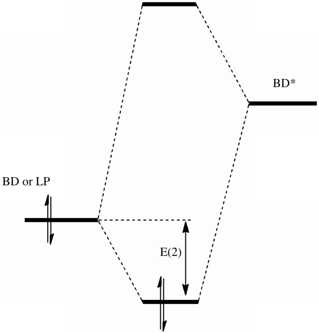
This is exactly the form of the Klopman-Salem diagram you may well recollect from 2nd year lectures, and also repeated in the stereo-electronisc course. But we have now made progress, by using the NBO expressions, we can obtain an exact value for the value of the quantity E(2).
When this is done for the two dioxepins discussed in case study 1, the following results (at the B3LYP/6-31G(d) level, but that need not concern us here) are obtained for the stable form;
The only two large E(2) terms (~15.5 kcal/mol) are between an oxygen LP and a C-O BD* involving the adjacent oxygen. They correspond exactly to the two antiperiplanar interactions we first noticed by visualisation, but now we can precisely quantify these interactions.
For the unstable isomer, only one large E(2) term is found (13.4); the other (7.5) is now significantly reduced because the orientation is no longer exactly antiperiplanar. The molecule is less stabilised and the two C-O bonds are no longer equal in length.

NBO analysis is very useful in a variety of situations, and is increasingly found in the literature. For example, it can be used to rationalise the gauche preference of 1,2-difluoroethane, and many others. Such E(2) NBO terms are thought to indicate useful chemistry down to energies of ~4 kcal/mol, and ones as high as 130 kcal/mol have been found (~15 is however typical of the anomeric effect).

Case Study 4 Revisited: Bonds can be Non-Classical (i.e. span 3 centres)

We saw before how the angular distorsion at a carbocation can be modelled using Molecular Mechanics. But this presupposes that we know exactly where the σ bonds actually are. Normally, this is not a problem, but in fact it can be so with carbocations, since they are electron deficient systems, and hence can adopt quite creative ways of offsetting this shortage of electrons! In Case study 7, we saw how we could use molecular orbital theories to predict the polarisation of π bonds. We can now go one stage further and predict how σ bonds might be polarized in an electron deficient system.

The reaction above gives two isomers, arising out of the intermediacy of a norbornyl cation, followed by quenching with bromide anion. The stereochemistry for the 1,3 isomer corresponds to syn whilst that of the 1,2 isomer is anti. Given the steric environment of Br is rather large, the observed 1,3 stereochemistry seems rather surprising. Can we explain it?

Both Br⁺ and C⁺ can form bridging species, the latter being a so called non-classical species, as well as more conventional unbridged (classical) forms. Four isomers are therefore possible 1-4. Four further isomers 5-8 derive from the alternate stereochemistry of the bromine.

System	Relative energy	Digital Repository
	0.0	10042/to-65
	1.0	10042/to-63
	8.1	10042/to-64
	2.5	10042/to-69
	1.0	10042/to-66
	0.0	10042/to-67
	-	-

These non-classical species have bonding which cannot easily be described as single/double etc, and hence cannot be studied by MM methods. [The non-classical norbornyl cation had a fascinating and very controversial history during the 1950s to 1970s, some people arguing that it did not exist, and others that it did. For years, a "definitive experiment" to distinguish whether the norbornyl cation was classical or non-classical was sought. The argument was in the event actually settled by spectroscopic rather than chemical experiments (photoelectron and ¹³C). Nowadays, very probably the argument would actually be settled by modelling!] The systems are small enough to be studied at a reasonable level of theory; we have chosen B3LYP/cc-pVTZ in this case. As we found with the primary carbonium ion (Case study 2), the classical carbonium ions cannot be found in the potential surface after geometry optimisation, and only 3,4,7,8 can be located. In 4, the atom coloured orange is electron deficient, and it can rectify this by sharing either with a lone electron pair from the adjacent bromine (structure 3) or by persuading the electron pair occupying the C-C bond shown in green for structure 3 to indulge in a ménage à trois (structure 4). The green "C-C bonds" shown in the Jmol rendition of structure 4 are NOT two electron bonds; rather the two electrons are shared more or less equally by three carbons (more of a ménage à cinq), in what is called a 3-centre-2-electron bond. Species 7 and 8 come out rather higher in energy (For a critical point analysis, see DOI: 10.1016/S0166-1280(98)00625-3)

Now, we can explain the products formed by this reaction. Opening of 4 would lead to 1,3 dibromination with syn di-bromo stereochemistry because attack at the yellow carbon atom (by Br^-) can only occur from one direction (attack at the orange carbon is sterically too hindered). Opening of 3 (at e.g. the orange carbon) would lead to 1,2 dibromination with anti di-bromo stereochemistry. Thus the two observed products can only really be explained by invoking two different non-classical intermediates of very similar energy.

What happens when Br is replaced by other halogens? When the halogen is F, steric factors become much less important, and the electronic impact of such an electron withdrawing group becomes paramount. Thus in the equatorial position, the F withdraws so much electron density from the anti-periplanar non-classical ion that the C⁺ localises as far from the F as possible. When in the axial position, the F is now orthogonal to the carbocation, and the non-classical bridge is preserved!

Return to main course page|| Back to Visualisation| Back to Mechanics|On to Transition states| On to Advanced|