. If you are
following these instructions using the tutorial data for the
structure shown below, use the Bruker option
. If you are
following these instructions using the tutorial data for the
structure shown below, use the Bruker option  .
.Modern NMR identification uses a range of techniques to provide connectivity and stereochemical information about molecules. In this tutorial, a range of datasets deriving from these techniques are stored on a network file server. This tutorial illustrates how this data can be processed using appropriate software to provide structural information.
Data from two principle sources is available for processing,
the Bruker spectrometers and the Jeol system. The latter is
used for running all Student (1D) NMR samples, the former for
more complex (often 2D) data sets. If you are following these
instructions to process your laboratory acquired data, use the
Jeol option. If you are
following these instructions using the tutorial data for the
structure shown below, use the Bruker option .
Various programs are available for processing NMR data:
Mestrec1D (filename
mestrecXY.exe, where XY is the current version number)Mestrec2D (filename
mestrecnd.exe)SpecNMR (filename
spexnmr.exe)To access these programs, proceed as follows:

 On MacOS X, run the
Remote
Desktop connection program (found in Applications or the
Dock, icon same as above) and specify
chas.ch.ic.ac.uk as the remote
application servers. You will enter a standard Windows
environment, and Mestre-C, SpecNMR and NMR Service icons
should be seen on the desktop or from the Start menu. You
must remember to log out of these servers when you finish: do
not leave yourself logged in, or just quit the remote desktop
program without so logging out.The Bruker tutorial
datasets for the compound shown at the left are located on
the local in a folder called NMR_Data, which
contains the following subfolders:
On MacOS X, run the
Remote
Desktop connection program (found in Applications or the
Dock, icon same as above) and specify
chas.ch.ic.ac.uk as the remote
application servers. You will enter a standard Windows
environment, and Mestre-C, SpecNMR and NMR Service icons
should be seen on the desktop or from the Start menu. You
must remember to log out of these servers when you finish: do
not leave yourself logged in, or just quit the remote desktop
program without so logging out.The Bruker tutorial
datasets for the compound shown at the left are located on
the local in a folder called NMR_Data, which
contains the following subfolders: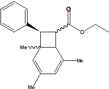 1H is the 400 MHz 1H
spectrum13C is the
corresponding 13C dataCOSY-2D is the 1H/1H
correlated 2D dataH-C-2D is the 1H/13C
correlated 2D dataNOE is the 1H NOE
experimentsThe 1D datasets
should be opened with the MestreC23 program, the 2D datasets
with the MestrecND program (both located on C:\Mestrec or
D:\Mestrec). Proceed as followsFrom the 1H sub-folder of NMR_Data,
browse to the file called FID. Note that for this
file, you should select a Bruker UXNMR file type.
1H is the 400 MHz 1H
spectrum13C is the
corresponding 13C dataCOSY-2D is the 1H/1H
correlated 2D dataH-C-2D is the 1H/13C
correlated 2D dataNOE is the 1H NOE
experimentsThe 1D datasets
should be opened with the MestreC23 program, the 2D datasets
with the MestrecND program (both located on C:\Mestrec or
D:\Mestrec). Proceed as followsFrom the 1H sub-folder of NMR_Data,
browse to the file called FID. Note that for this
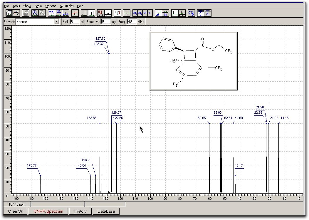
file, you should select a Bruker UXNMR file type.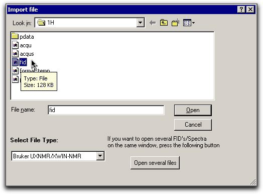 From process, select
Fourier transformView/Set limits to
view spectrum between predefined values of the chemical
shift.Use Tools/Reference
and Tools/Integrate, followed by a dragging out of the area
of spectrum to be integrated.Use +/- from the
toolbar to change height of spectrumThere are numerous
other options, which you should explore yourself. The results
look akin to this;
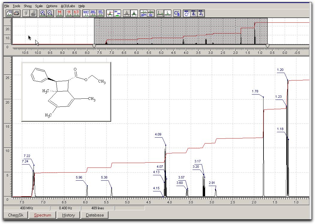
From process, select
Fourier transformView/Set limits to
view spectrum between predefined values of the chemical
shift.Use Tools/Reference
and Tools/Integrate, followed by a dragging out of the area
of spectrum to be integrated.Use +/- from the
toolbar to change height of spectrumThere are numerous
other options, which you should explore yourself. The results
look akin to this;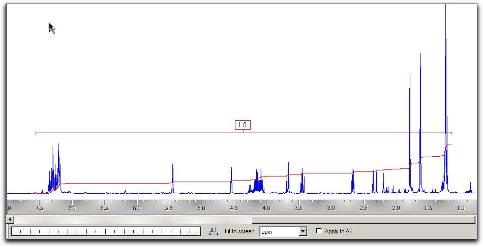 Repeat for the folder
NOE/4-17/pdata/2/1r to see various nOe experiments. The
different spectra relate to different pre-irradiations at
selected frequencies, and show the difference spectrum
resulting.For the 2D plots,
proceed as follows;Using MestrecND, go
to eg COSY-2D and open the file ser.Process/Fourier
transform/Apodise/SineBell/Apply along t2. You should now see
a display comprising a series of vertical stripes. From the
menu, change the size to four times its initial value (zero
filling eg 256 to 1k) and Apply along t1. The result will be
a 2D spectrum. Hit + a few times to increase the size of the
contours. Use Tools/Reference F1 and Reference F2 to set the
chemical shift to known values, ie TMS. Proton COSY spectra
usually look better if symmetrised (Process menu) and forced
to be square.Go to H-C-2D and do
the same. In each case the 1H/1H or 1H/13C spectrum is
displayed along one frequency axis. The interpretation is
that cross peaks in 1H/1H correlation indicate 1H-1H coupling
and likewise for 1H/13C.When you have a
spectrum to your liking, Copy data to the clipboard and paste
into Microsoft Word or other word processor for inclusion in
your report. Do not attempt direct printing, there are no
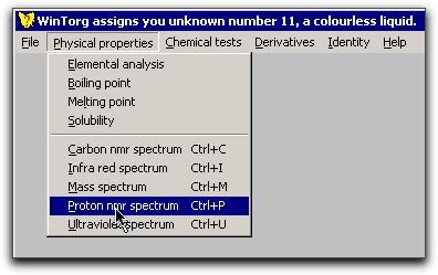
printers provided for the purpose. The Jeol datasets
derived from samples run as part of laboratory experiments
are located in a network drive called 270teaching,
subdirectory data on "chnmr3" in the domain CH1. You may find this
folder mounted on the "Resonance" network drive (270teaching on 'Chnmr3' (R:) The
spectra should appear there after the sample has been run.
Note carefully the spectrum code assigned to you. Run the SpecNMR
program located in D:\SpecNMR (there should be a shortcut on the
desktop). Invoke File/Open,
select Jeol Delta Format as the file type
() and click on Drives and browse
to R:\Data\...appropriate sub-folders,
Click OK/finish. A list of available files listed in the file
dialog box appears. Select the one you want. The screen should
shown an FID (Free induction decay). Select
Process/FT+Phase/OK. An (unphased) spectrum appears. From the Phase
floating pane and P0 set, move the slider labelled degrees
until the marked peak appears properly phased. Then select P1
and again move the slider until the rest of the spectrum
looks properly phased. Finish with Apply. The spectrum can be
expanded by dragging out a box for expansion. Analyse/Integrate.
Hold the right mouse button down (on a Mac, Control/Shift)
and pull out a region on the spectrum to integrate. Repeat as
often as necessary. Process/Calibrate to
set the reference. Right click to set the point on the
spectrum whose chemical shift you know (i.e. TMS) and click
OK. If you cannot find a peak whose position you know, enter
8096 (assuming your FID is a 16k one)
into the data box and 5.00ppm into the chemical shift box and
click OK. The result should be fairly accurate. The spectrum should look similar to:
Repeat for the folder
NOE/4-17/pdata/2/1r to see various nOe experiments. The
different spectra relate to different pre-irradiations at
selected frequencies, and show the difference spectrum
resulting.For the 2D plots,
proceed as follows;Using MestrecND, go
to eg COSY-2D and open the file ser.Process/Fourier
transform/Apodise/SineBell/Apply along t2. You should now see
a display comprising a series of vertical stripes. From the
menu, change the size to four times its initial value (zero
filling eg 256 to 1k) and Apply along t1. The result will be
a 2D spectrum. Hit + a few times to increase the size of the
contours. Use Tools/Reference F1 and Reference F2 to set the
chemical shift to known values, ie TMS. Proton COSY spectra
usually look better if symmetrised (Process menu) and forced
to be square.Go to H-C-2D and do
the same. In each case the 1H/1H or 1H/13C spectrum is
displayed along one frequency axis. The interpretation is
that cross peaks in 1H/1H correlation indicate 1H-1H coupling
and likewise for 1H/13C.When you have a
spectrum to your liking, Copy data to the clipboard and paste
into Microsoft Word or other word processor for inclusion in
your report. Do not attempt direct printing, there are no
printers provided for the purpose. The Jeol datasets
derived from samples run as part of laboratory experiments
are located in a network drive called 270teaching,
subdirectory data on "chnmr3" in the domain CH1. You may find this
folder mounted on the "Resonance" network drive (270teaching on 'Chnmr3' (R:) The
spectra should appear there after the sample has been run.
Note carefully the spectrum code assigned to you. Run the SpecNMR
program located in D:\SpecNMR (there should be a shortcut on the
desktop). Invoke File/Open,
select Jeol Delta Format as the file type
() and click on Drives and browse
to R:\Data\...appropriate sub-folders,
Click OK/finish. A list of available files listed in the file
dialog box appears. Select the one you want. The screen should
shown an FID (Free induction decay). Select
Process/FT+Phase/OK. An (unphased) spectrum appears. From the Phase
floating pane and P0 set, move the slider labelled degrees
until the marked peak appears properly phased. Then select P1
and again move the slider until the rest of the spectrum
looks properly phased. Finish with Apply. The spectrum can be
expanded by dragging out a box for expansion. Analyse/Integrate.
Hold the right mouse button down (on a Mac, Control/Shift)
and pull out a region on the spectrum to integrate. Repeat as
often as necessary. Process/Calibrate to
set the reference. Right click to set the point on the
spectrum whose chemical shift you know (i.e. TMS) and click
OK. If you cannot find a peak whose position you know, enter
8096 (assuming your FID is a 16k one)
into the data box and 5.00ppm into the chemical shift box and
click OK. The result should be fairly accurate. The spectrum should look similar to: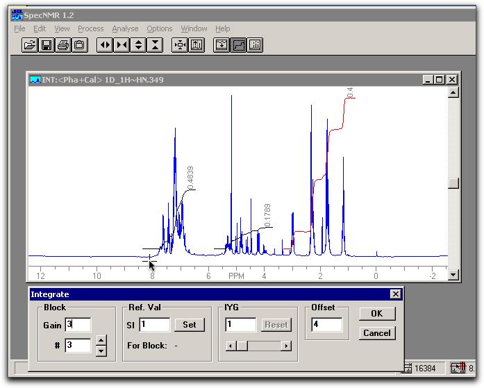 Edit/copy to clipboard
and Paste into Word. Save the Word file either to a removable
device (e.g. Pendrive) or to your Network H: drive.
Edit/copy to clipboard
and Paste into Word. Save the Word file either to a removable
device (e.g. Pendrive) or to your Network H: drive.The tutorial relates the following compound, but you should
apply the procedure to your own data.